1. What's FM?
The FM, full name Factorization Machine, was proposed by STEFFEN RENDLE of the University ofKonstanz in 2012
2. What improvements have been made to FM
Let's look at the original quote from FM's paper
In contrast to SVMs, FMs model all interactions between variablesusing factorizedparameters.Thus they are able to estimate interactionseven inproblems with huge sparsity(like recommender systems) where SVMs fail.
Meaning: In contrast to SVM, FMs use decomposition parameters to model all interactions between variables. As a result, they are able to predict the interactions between variables even inproblems with huge sparsity (e.g., recommender systems), a domain where SVM fails. In other words, FM employs a technique that is able to find the interactions of variables in sparseproblems. One problem with logistic regression is that it is difficult to learn the weights of sparsecombinatorial features. Let's first look at why logistic regression is unable to learn the weights of sparse combinatorial features from a modeling perspective. Suppose the single combined feature of logistic regression is,which represents that the user is female and likes to get up at 12 o'clock in the middle of the night to eat fish. This feature is very sparse when you think about it, very few users have such odd habits, and we want to learn the weights of this feature. Let's think about the weight update formula for logistic regression,
\theta_j := \theta_j - \alpha\sum_{i=1}^{m}(h_\theta(x^{(i)}) - y^{(i)}))*x_{j}^{(i)}You can take a look at the last item,$x_j^{(i)}$,if most of this item is 0, then the gradient descent of is very small in each step, and there is no way to get the weights. FM solves this problem for logistic regression, especially in recommendation & advertisement scenarios, where sparse features are very.
The improvement of FM is to say that the weight of the combination of features becomes the dot product of two groups and feature v-vectors, instead of directly calculating the group and the weight, which solves the problem of training, because even if the group and the features do not
appear, but the two features have appeared separately, and the group and the features can also get the weight. As an example, for example, the user is female and likes to eat fish at 12 midnight, this group and feature is rarely seen, but split, the user is female and the user likes to eat fish at 12
midnight, the probability of these two features appearing separately is quite a bit larger than the group and appear, we multiply the v-vector of the user being female and the v-vector of the user liking to eat fish at 12 o'clock by a dot to get the weights of the combined features. Let's look at what else the original FM paper said.

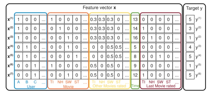
In sparse settings, there is usually not enough data to estimate interactions between variables directly and independently. Factorization machines can estimate interactions even in these settings well because they break the independence of the interaction parameters by factorizing them. In general this means that the data for one interaction helps also to estimatethe parameters for related interactions. We will make the idea more clear with an example from the data in figure 1. Assume we want to estimate the interaction between Alice (A) and Star Trek (ST) for predicting the target y (here the rating).Obviously, there is no case x in the training data where both variables xA and xST are non-zero and thus a direct estimate would lead to no interaction (wA,ST = 0). But with the factorized interaction parameters⟨vA,vST⟩ we can estimate the interaction even in this case. First of all, Bob and Charlie will have similar factor vectors vB and vC because both have similar interactions with Star Wars (vSW) for predicting ratings – i.e. ⟨vB,vSW⟩ and ⟨vC,vSW⟩ have to be similar. Alice (vA) will have a different factor vector from Charlie (vC) because she has different interactions with the factors of Titanic and Star Wars for predicting ratings. Next, the factor vectors of Star Trek are likely to be similar to the one of Star Wars because Bob has similar interactions for both movies for predicting y. In total, this means that the dot product (i.e. the interaction) of the factor vectors of Alice and Star Trek will be similar to the one of Alice and Star Wars – which also makes intuitively sense.
3.How FM achieved these improvements
Form of FM
Let's first look at the formula for FM
y(x):= w_0+\sum_{i=1}^n + \sum_{i=1}^{n}\sum_{j=i+1}^n<V_i,V_j>x_ix_jincluded among these
w_0\in R, w\in R^n,V\in R^{n\times k}n is the number of features, and k is the dimension of the v-vector. To make this easier to understand, we define a data matrix, and a v-matrix. The data matrix is 4 by 3, and the v-matrix is 3 by 2. You can see that the number of columns in the data is the number of rows in the v-matrix.
data=
\left[
  \begin{matrix}
   x_{11} & x_{12} & x_{13} \\
   x_{21} & x_{22} & x_{23} \\
   x_{31} & x_{32} & x_{33} \\
    x_{41} & x_{42} & x_{43}
  \end{matrix}
  \right]
This is a data matrix with four rows of data and three features.
 V=
\left[
  \begin{matrix}
   v_{11} & v_{12} \\
   v_{21} & v_{22}  \\
   v_{31} & v_{32}
  \end{matrix}
  \right]
This is the V matrix, each type of feature corresponds to a row of V vectors with 2 bits for each type of feature. For example, we want to compute ,which is the combination of the first type of feature and the second type of feature The formula is
<V_i,V_j> = \sum_{f=1}^{k}v_{i,f}v_{j,f}To put it bluntly.
v_{11}*v_{21}+v_{12}*v_{22}The core of FM is to train the V-matrix and calculate the intersection of the V-matrix, but if you
calculate them one by one as in the above equation, the computation is O(kn).
4. Cross Term Expansion of FM
The process of pushing back is as follows:
\begin{aligned}
\sum_{i=1}^{n-1} \sum_{j=i+1}^{n}\left(\mathbf{v}_{i}^{\top} \mathbf{v}_{j}\right) x_{i} x_{j} &=\frac{1}{2}\left(\sum_{i=1}^{n} \sum_{j=1}^{n}\left(\mathbf{v}_{i}^{\top} \mathbf{v}_{j}\right) x_{i} x_{j}-\sum_{i=1}^{n}\left(\mathbf{v}_{i}^{\top} \mathbf{v}_{i}\right) x_{i} x_{i}\right) \\
&=\frac{1}{2}\left(\sum_{i=1}^{n} \sum_{j=1}^{n} \sum_{l=1}^{k} v_{il} v_{jl} x_{i} x_{j}-\sum_{i=1}^{n} \sum_{l=1}^{k} v_{il}^{2} x_{i}^{2}\right) \\
&=\frac{1}{2} \sum_{l=1}^{k}\left(\left(\sum_{i=1}^{n}\left(v_{il} x_{i}\right) \sum_{j=1}^{n}\left(v_{jl} x_{j}\right)\right)-\sum_{i=1}^{n} v_{il}^{2} x_{i}^{2}\right) \\
&=\frac{1}{2} \sum_{l=1}^{k}\left[\left(\sum_{i=1}^{n} v_{il} x_{i}\right)^{2}-\sum_{i=1}^{n} v_{il}^{2} x_{i}^{2}\right]
\end{aligned}
I'll explain the FM algorithm in terms of multiplication of matrices.
data=
\left[
  \begin{matrix}
   x_{11} & x_{12} & x_{13} \\
   x_{21} & x_{22} & x_{23} \\
   x_{31} & x_{32} & x_{33} \\
    x_{41} & x_{42} & x_{43}
  \end{matrix}
  \right]
V=
\left[
\begin{matrix}
v_{11} & v_{12} \\
v_{21} & v_{22} \\
v_{31} & v_{32}
\end{matrix}
\right]Let's take a look at these two matrices,First of all, the above formula works on each row of the DATA matrix, suppose we want to count the first row, that is ,suppose we have the V matrix, to calculate the value of the V characteristic part of the first row of data. The first line of the above formula looks like this,
0.5((V_1V_1x_{11}x_{11}+V_1V_2x_{11}x_{12}+V_1V_3x_{11}x_{13}+...+V_3V_3x_{13}x_{13}) \\- (V_1V_1x_{11}x_{11}+V_2V_2x_{22}x_{22}+V_3V_3x_{33}x_{33})Where V_1 is [v_{11},v_{12},v_{13}] ,so V_1V_1x_{11}x_{11} is
(v_{11}*v_{11}+v_{12}*v_{12}+v_{13}*v_{13})*x_{11}x_{11}Next we look at the second line of the formula.
The second line of the formula is the one that expands the formula as I did above, and in our case, k is 2.
Next, let's look at the formula of the third line, which is still quite critical. I'm sure the author of fm pushed back to this point and must have still put some thought into it.First of all for v-vector multiplication, each multiplication, for each must be the same column of multiplication, for our example, must be [v_{11},v_{21},v_{31}]^T play together ,[v_{12},v_{22},v_{32}]^T play together.so that the equation can be split. We first consider the case ,ie. [v_{11},v_{21},v_{31}]^T these three brothers play together, and Eq
(v_{11}x_{11}+v_{21}x_{12}+v_{31}x_{13})*(v_{11}x_{11}+v_{21}x_{12}+v_{31}x_{13})\\ - (v_{11}v_{11}x_{11}x_{11}+v_{21}v_{21}x_{12}x_{12}+v_{31}v_{31}x_{13}x_{13})When k = 2, which is [v_{12},v_{22},v_{32}]^T the three brothers play together, the equation is
(v_{12}x_{11}+v_{22}x_{12}+v_{32}x_{13})*(v_{12}x_{11}+v_{22}x_{12}+v_{32}x_{13}) \\- (v_{12}v_{12}x_{11}x_{11}+v_{22}v_{22}x_{12}x_{12}++v_{32}v_{32}x_{13}x_{13})These two together make up the third line of the formula, and the fourth line changes the
equation into the form of a square term.
5. Solving for the weights of FM
Assuming we use FM to categorize, using cross-entropy loss, the pushback process is essentially the same as logistic regression.
h_{\theta}(x)-g\left(\theta^{T} x\right)=\frac{1}{1+e^{-\theta^{T} x}}We assume that the training samples are independent of each other, then the likelihood function expression is:
\begin{aligned}
L(\theta) &=p(\vec{y} | X ; \theta) \\
&=\prod_{i=1}^{m} p\left(y^{(i)} | x^{(i)} ; \theta\right) \\
&=\prod_{i=1}^{m}\left(h_{\theta}\left(x^{(i)}\right)\right)^{y^{(i)}}\left(1-h_{\theta}\left(x^{(i)}\right)\right)^{1-y^{(i)}}
\end{aligned}
Again take log for the likelihood function and convert:
\begin{aligned}
\ell(\theta) &= \log L(\theta) \\
&= \sum_{i=1}^{m} y^{(i)} \log \left(h\left(x^{(i)}\right)\right)+\left(1-y^{(i)}\right) \log \left(1-h\left(x^{(i)}\right)\right)
\end{aligned}
The transformed likelihood function takes a partial derivative with respect to θ. Here we take the case of only one training sample as an example:
\begin{aligned}
\frac{\partial}{\partial \theta_{i}} t(\theta) &=\left(\frac{1}{g\left(\theta^{T} x\right)}\left(1-y\right) \frac{1}{1-g\left(\theta^{T} x\right)}\right) \frac{\partial}{\partial \theta_{i}} g\left(\theta^{T} x\right) \\
&=\left(\frac{1}{g\left(\theta^{T} x\right)}-\left(1-y\right) \frac{1}{1-g\left(\theta^{T} x\right)}\right) g\left(\theta^{T} x\right)\left(1-g\left(\theta^{T} x\right)\right) \frac{\partial}{\partial \theta_{i}} \theta^{T} x \\
&=\left(y\left(1-g\left(\theta^{T} x\right)\right)-\left(1-y\right) g\left(\theta^{T} x\right)\right) x_{i} \\
&=\left(y-h_{\theta}(x)\right) x_{i}
\end{aligned}
This can also be seen as a derivation of the FM model, specifically for the m,v part only need to replace x_j in (y-h_\theta(x))x_j,beause x_j is \frac{\partial}{\partial\theta_{j}}\theta^Tx .we need to replace it with \frac{\partial}{\partial v_{jl}}\sum^n_{i=1}\sum^n_{j=i+1}.This paper begs for us.
\frac{\partial g}{\partial \theta}=\left\{\begin{array}{ll}
1, & \text { if } \theta=w_{0} \\
x_{i}, & \text { if } \theta=w_{i} \\
x_{i} \sum_{j=1}^{n} v_{j} x_{j}-v_{i} x_{i}^{2}, & \text { if } \theta=v_{i}
\end{array}\right.
6.Python implementation of FM
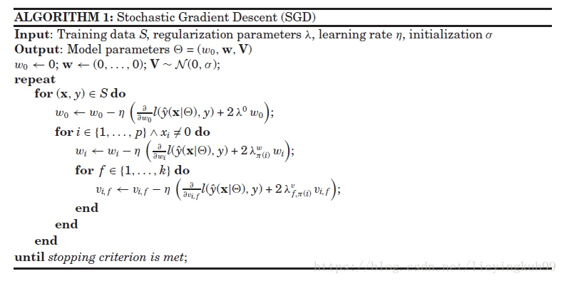
Stochastic Gradient Descent Implementation Steps:

this is someone else's implementation, using stochastic gradient descent method, but the original implementation for the class label is -1 and 1, I here re-derivation of the loss function, for the class label is 0 and 1, the original code is python2, changed to python3
#!/usr/bin/env python3
# -*- coding: utf-8 -*-
"""
Created on Wed Mar 27 17:03:47 2019

@author: sean.zhang
"""

from __future__ import division
from math import exp
import numpy as np
from random import normalvariate  # 正态分布
from datetime import datetime
import pandas as pd

trainData = 'diabetes_train.txt'   #请换为自己文件的路径
testData = 'diabetes_test.txt'

def preprocessData(data):
    feature=np.array(data.iloc[:,:-1])   #取特征
    label=data.iloc[:,-1] #取标签并转化为 1 0
    #将数组按行进行归一化
    zmax, zmin = feature.max(axis=0), feature.min(axis=0)
    feature = (feature - zmin) / (zmax - zmin)
    label=np.array(label)
    return feature,label

def sigmoid(inx):
    #return 1. / (1. + exp(-max(min(inx, 15.), -15.)))
    return 1.0 / (1 + exp(-inx))

def getAccuracy(dataMatrix, classLabels, w_0, w, v):
    m, n = dataMatrix.shape
    allItem = 0
    error = 0
    result = []
    for x in range(m):   #计算每一个样本的误差
        allItem += 1
        inter_1 = np.dot(dataMatrix[x] , v)
        inter_2 = np.multiply(dataMatrix[x], dataMatrix[x]) *np.multiply(v, v)
        interaction = sum(np.multiply(inter_1, inter_1) - inter_2) / 2.
        p = w_0 + dataMatrix[x] * w + interaction  # 计算预测的输出

        pre = sigmoid(p[0, 0])
        result.append(pre)

        if pre < 0.5 and classLabels[x] == 1.0:
            error += 1
        elif pre >= 0.5 and classLabels[x] == 0.0:
            error += 1
        else:
            continue

    return (result,float(error) / allItem)

#%%
from numpy import random
train=pd.read_csv(trainData)
test = pd.read_csv(testData)
dataTrain, labelTrain = preprocessData(train)
dataTest, labelTest = preprocessData(test)
date_startTrain = datetime.now()
dataMatrix = np.mat(dataTrain)
m, n = dataMatrix.shape   #矩阵的行列数,即样本数和特征数
alpha = 0.01
k=19
# 初始化参数
# w = random.randn(n, 1)#其中n是特征的个数
w = np.zeros((n, 1))      #一阶特征的系数
w_0 = 0.
iters = 500
classLabels = labelTrain
v = normalvariate(0, 0.2) * random.random((n, k))   #即生成辅助向量,用来训练二阶交叉特征的系数
for it in range(iters):
    errs = 0.0
    for x in range(m):  # 随机优化,每次只使用一个样本
        inter_1 = np.dot(dataMatrix[x], v) #一行n列
        inter_2 = np.multiply(dataMatrix[x], dataMatrix[x]) * np.multiply(v, v)  #二阶交叉项的计算。 一行n列
        interaction = sum(np.multiply(inter_1, inter_1) - inter_2) / 2.       #二阶交叉项计算完成 1行1列
        p = w_0 + np.dot(dataMatrix[x] ,w) + interaction  # 计算预测的输出,即FM的全部项之和
        err = (classLabels[x] - sigmoid(p[0, 0]))
        errs += err

        w_0 = w_0 +alpha * err
        for i in range(n):
            if dataMatrix[x, i] != 0:
                w[i, 0] = w[i, 0] +alpha * err * dataMatrix[x, i]
                for j in range(k):
                    v[i, j] = v[i, j]+ alpha * err * (
                    dataMatrix[x, i] * inter_1[0, j] - v[i, j] * dataMatrix[x, i] * dataMatrix[x, i])
    print(it,errs)
#%%
result,errRate = getAccuracy(np.mat(dataTest), labelTest, w_0, w, v)
print( "测试准确性为:%f" % (1 - errRate))
from sklearn import metrics
fpr, tpr, thresholds = metrics.roc_curve(labelTest, result, pos_label = 1)
print(metrics.auc(fpr, tpr))